Offline Setting

SPREAD is particularly well suited for offline optimization scenarios. In this setting, the objective functions are not available during optimization. Instead, each task provides a fixed dataset of the form (X, F(X)), and the diffusion model is trained solely on this static dataset.

We provide several benchmark tasks in Test Problems, whose datasets can be downloaded from Off-MOO-Bench.

In this example, we use the rocket injector design task (RE37), which is a three-objective problem.

import numpy as np
import torch

# Import the SPREAD solver
from moospread import SPREAD

# Import a test problem
from moospread.tasks import RE37

# Define the problem
problem = RE37(ref_point=[0.99, 0.96, 0.99]) # reference point from our paper

When initializing the SPREAD solver, the parameter mode must be set to "offline", and the training dataset (X, y) must be provided via the dataset argument. Setting timesteps to values around 1000 is typically sufficient to obtain good performance.

You may also use a custom surrogate model architecture by specifying surrogate_model and its corresponding training function via train_func_surrogate. By default, moospread uses the MultipleModels surrogate from Offline Multi-Objective Optimization, trained on the provided static dataset as a proxy for the objective functions. In offline optimization, dataset points are commonly normalized using z-score or min–max scaling. moospread provides this functionality through the offline_normalization_method argument. Valid values are "z_score", "min_max", and None. The default is "z_score".

# Load data
X = np.load("/path_to_data/re37-x-0.npy")
y = np.load("/path_to_data/re37-y-0.npy")

X = torch.from_numpy(X).float()
y = torch.from_numpy(y).float()

# Initialize the SPREAD solver
solver = SPREAD(
    problem,
    dataset=(X, y),
    num_blocks=2,
    timesteps=1000,
    num_epochs=1000,
    train_tol=100,
    train_tol_surrogate=100,
    mode="offline",
    model_dir="./model_dir/",
    proxies_store_path="./proxies_dir/",
    seed=2026,
    verbose=True
)

If no dataset is provided, the SPREAD solver must have access to the true objective functions in order to generate a training dataset using Latin Hypercube Sampling (LHS). In this case, the data_size argument must be specified, allowing an online problem to be treated as an offline task.

To solve the problem, specify the number of solutions to generate using the num_points_sample argument. If the solver is reused with the same initialization, retraining of both the diffusion model and the surrogate models can be avoided by setting load_models=True. In the offline setting, we recommend the following parameter choices:

• For bi-objective problems:

  • rho_scale_gamma = 0.9 / 0.1 / 0.0001

  • eta_init = 0.9 / 0.5 / 0.02

  • lr_inner = 0.9 / 0.002

• For problems with more than two objectives:

  • rho_scale_gamma = 0.001 / 0.0001

  • eta_init = 0.1 / 0.01

  • lr_inner = 0.9

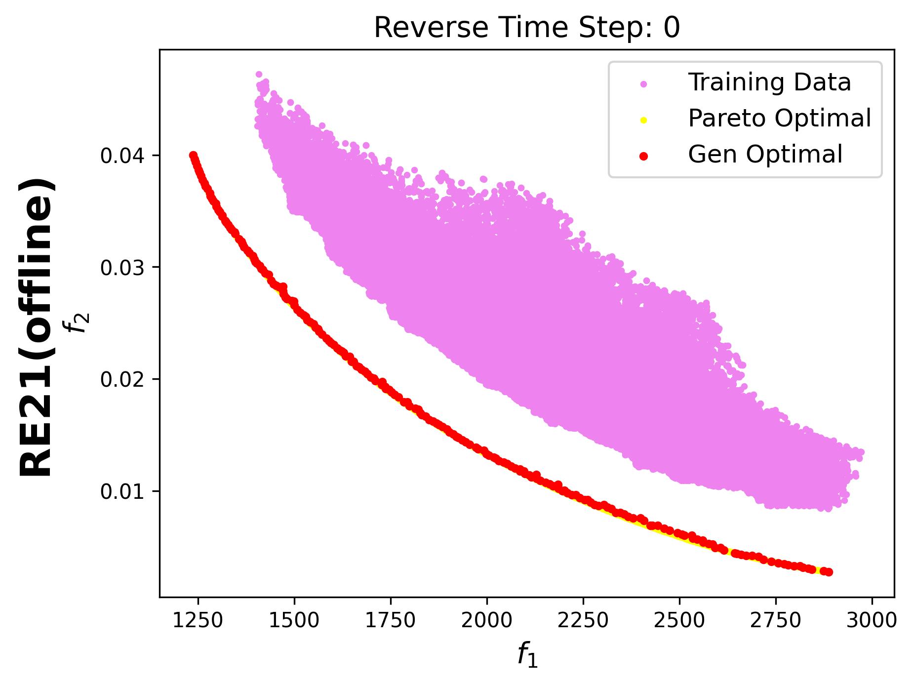
If you do not need intermediate Pareto fronts, set iterative_plot=False. When enabled, plot_dataset=True allows you to display the static dataset alongside the generated solutions, making it easier to evaluate their quality.

# Solve the problem
res_x, res_y = solver.solve(
    num_points_sample=200,
    rho_scale_gamma=0.001,
    eta_init=0.1,
    lr_inner=0.9,
    iterative_plot=True,
    plot_period=10,
    plot_dataset=False,
    max_backtracks=25,
    save_results=True,
    samples_store_path="./samples_dir/",
    images_store_path="./images_dir/"
)

Since in this example we enable iterative_plot, we can visualize the generative process using the images saved in images_store_path (see Visualization).

solver.create_video(
    image_folder="images_dir/RE37_offline",
    output_video="videos_dir/RE37_offline.mp4",
    total_duration_s=20.0,
    first_transition_s=2.0,
    fps=30,
)

Generative process

Final generated Pareto front

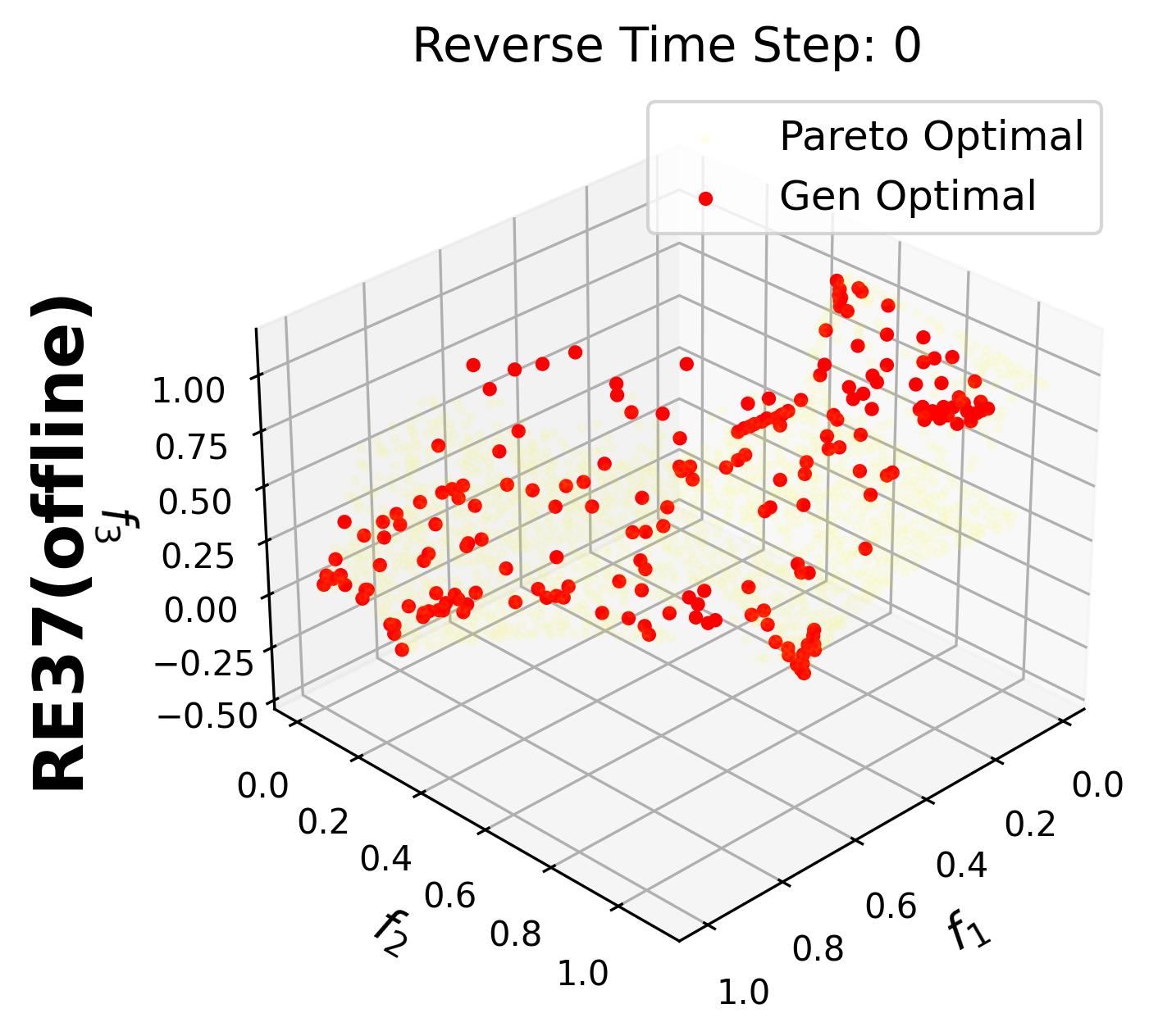
For 3-objective problems, plotting the training data may obscure the generated points. Therefore, in this example, we set plot_dataset=False for the RE37 problem.

Additionally, we visualize the generative process for the bi-objective RE21 problem, where the training data points are also displayed:

Generative process

Final generated Pareto front