MOBO Setting

In the multi-objective Bayesian optimization (MOBO) setting, the true objective functions are available but expensive to evaluate. Because the evaluation budget is typically small, collecting a large diffusion training dataset directly is infeasible. To address this limitation, moospread adopts the data-augmentation strategy of CDM-PSL. This approach produces a sufficiently large training dataset for the diffusion model while respecting the evaluation-budget constraints.

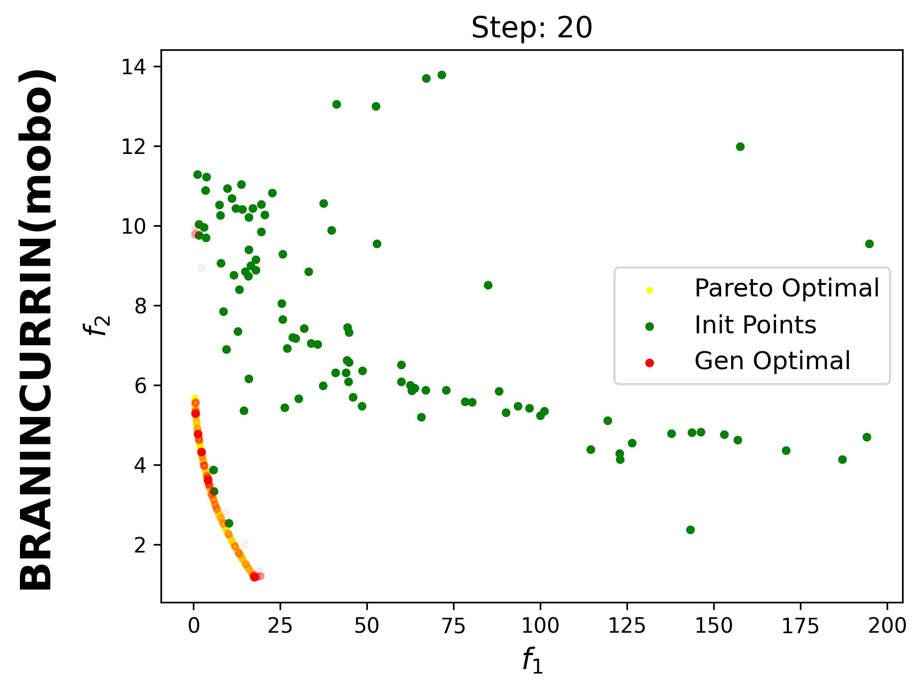
In this example, we use the Branin–Currin problem, which is a bi-objective benchmark task.

import numpy as np
import torch

# Import the SPREAD solver
from moospread import SPREAD

# Import a test problem
from moospread.tasks import BraninCurrin

# Define the problem
problem = BraninCurrin()

When initializing the SPREAD solver, the parameter mode must be set to "bayesian". Setting timesteps to a relatively small value (e.g., 25) is important to reduce computational cost and accelerate optimization.

You may use a custom surrogate model architecture by specifying surrogate_model and its corresponding training function via train_func_surrogate. By default, moospread uses Gaussian processes as surrogate models.

# Initialize the SPREAD solver
solver = SPREAD(
    problem,
    num_blocks=2,
    timesteps=25,
    num_epochs=1000,
    train_tol=100,
    mode="bayesian",
    model_dir="./model_dir/",
    seed=2026,
    verbose=True
)

To solve the problem, specify:

• the number of initial samples using n_init_mobo,

• the number of MOBO iterations using n_steps_mobo,

• the batch size selected at each step using batch_select_mobo, and

• the number of generations using spread_num_samp_mobo.

As shown in the experiments reported in the paper, using an auxiliary operator to escape local minima is beneficial. This can be enabled by setting use_escape_local_mobo=True.

In the MOBO setting, we recommend the following parameter choices:

• For bi-objective problems:

  • rho_scale_gamma = 0.9

  • eta_init = 0.9

  • lr_inner = 0.9

• For problems with more than two objectives:

  • rho_scale_gamma = 0.01 / 0.0001

  • eta_init = 0.9

  • lr_inner = 0.9 / 5e-4

If intermediate Pareto fronts are not required, set iterative_plot=False.

# Solve the problem
result_Xy, hv_all_value = solver.solve(
    rho_scale_gamma=0.9,
    eta_init=0.9,
    lr_inner=0.9,
    iterative_plot=True,
    plot_period=10,
    max_backtracks=25,
    save_results=True,
    samples_store_path="./samples_dir/",
    images_store_path="./images_dir/",
    n_init_mobo=100,
    use_escape_local_mobo=True,
    n_steps_mobo=20,
    spread_num_samp_mobo=25,
    batch_select_mobo=5
)

Since iterative_plot is enabled in this example, we can visualize the generative process using the images saved in images_store_path (see Visualization).

Here, the generated points are plotted after each MOBO step (1, 2, …, 20). Therefore, we need to set reverse=False.

solver.create_video(
    image_folder="images_dir/BraninCurrin_bayesian",
    output_video="videos_dir/BraninCurrin_bayesian.mp4",
    total_duration_s=20.0,
    first_transition_s=2.0,
    fps=30,
    reverse=False
)

Generative process

Final generated Pareto front

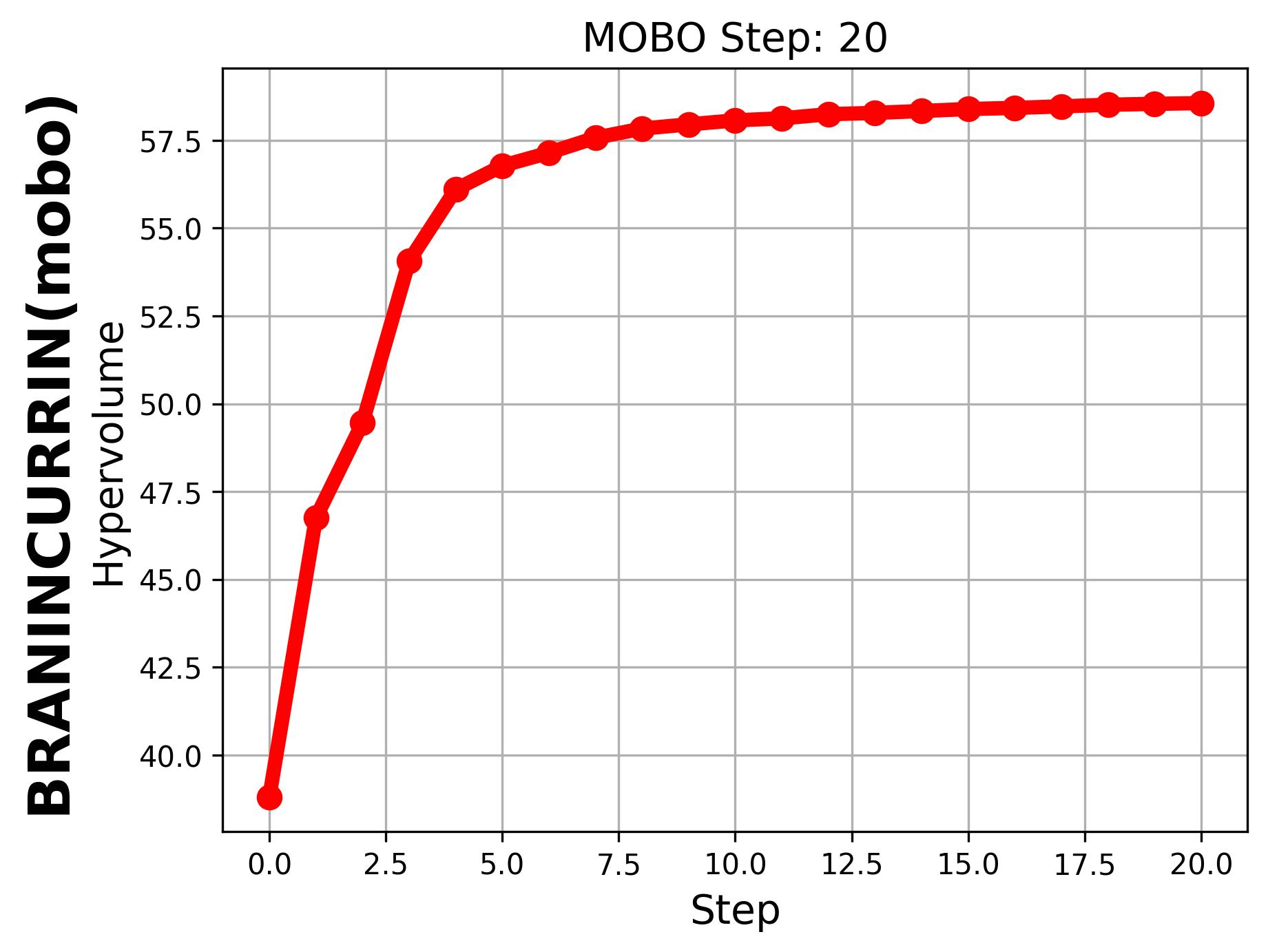
If we set hypervolume=True and provide hv_all_value_file="samples_dir/spread_BraninCurrin_T25_K20_FE100_seed=2026_bayesian_hv_results.pkl", we can visualize the evolution of the hypervolume.